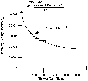
Figure A7.1 Observed failure time distribution for equipment with N=1,000 units on test
Once in a system, how long will an ASIC last? The answer remains uncertain. No deterministic models exist to predict microelectronics' lifetimes to a useful degree of accuracy. Also, though scientists have performed many empirical studies on simple microelectronics devices to determine their lifetimes, little empirical data exists for complex microelectronics (those with feature sizes less than 1.5 microns). Yet for the space industry, mission success depends upon reliability, since repair always proves either extremely expensive or impossible.
This section is broken into three parts. The first part provides a foundation by introducing basic ASIC reliability concepts. The second part discusses reliability modeling calculations and the most widely-used reliability modeling handbook, MIL-HDBK-217. The third part introduces the most common reliability test method: accelerated stress testing.
The reliability of an ASIC must take into account all types of failures, including defect-driven failures. Thus, determining an ASIC's reliability includes screening out defect-driven infant mortality failures and verifying that defect-driven end-of-life effects will not unacceptably shorten an ASIC's lifetime.
In general, models from these sources have not proven credible when predicting reliability quantitatively. Studies show that failure rates predicted by the above mentioned procedures can differ by over two orders of magnitude. However, if used in their proper perspective, these empirical models can usefully compare the reliability issues of two approaches to the same design.
The reliability modeling discussion is broken into two parts. The first part, "Basic Reliability Calculations," applies to all the empirical modeling procedures mentioned above. The second part, "Applying MIL-HDBK-217," goes into some detail about the most common empirical modeling handbook.
The cumulative distribution function is one of the central concepts in reliability. If a system starts to operate at time t=0, the probability that the system first fails at or before time t is given by the cumulative distribution function, F(t). If the failure time is denoted x, then
F(t) = Prob (x ≤ t)
F(t) has the following properties:
F(t) = 0 for t<0
0 ≤ F(t) ≤ F(t') for 0 ≤ t ≤ t'
F(t) → 1 for t → ∞
The survivor function S(t) gives the probability of surviving to time t without failure. It is closely related to F(t) by
S(t) = 1 - F(t)
Engineers sometimes refer to S(t) as the reliability function, R(t).


To better understand the reliability of some complex units, an
engineer tests 1000 units for 1000 hours. When a unit fails, the
engineer removes it from the test without repair. The engineer plots
the probability density function for the observed results as a bar plot
and fits a curve f(t) = 0.001e-0.001t to the data (see
figure A7.1). From this data, the engineer calculates the hazard rate,
the cumulative distribution function, and other information about the
units' survivability.

Figure A7.1 Observed failure time distribution for equipment with
N=1,000 units on test
Given the probability density function: f(t) = 0.001 e-
0.001t, then F(t) and S(t) may be readily calculated:

In this case, the hazard rate implies that the equipment failure rate
is 0.1 percent per hour.
The survivor function indicates the probability that a unit will survive throughout a given time. For instance, for t = 600 hours:
S(600) = e-0.001(600) = 0.55
Therefore, a unit has a 55 percent chance of surviving the first 600 operating hours. Equivalently, beginning with 1,000 units, the engineer expects 550 survivors in the first 600 hours.
The survivor function also serves to predict how many failures will occur within a specified time interval. For example, to determine the fraction of the original population that will fail between 600 and 800 hours, subtract S(800) from S(600):
S(600) - S(800) = e-0.001(600) - e-0.001(800) = 0.10
Thus, approximately 10 percent of the devices will fail during this interval.


All the models mentioned above use the constant failure rate reliability model:
R(t) = e-lt
where R(t) is the reliability of a device model at time t with a failure rate, l. The failure rate depends upon the device's environmental, physical, and operating characteristics assumed by the device model.
Each empirical reliability procedure has different device models, yielding vastly differing (and therefore not quantitatively credible) failure rates, as mentioned above. They all share a common language of factors that mathematically comprise the failure rates. These factors include: the quality factor, the environmental factor, the temperature acceleration factor, the voltage-stress factor, and the device or process learning factor.
Engineers assess a device's quality factor by inspecting and testing it. Each procedure has a different method for deriving the quality factor. The quality factor is especially important in MIL-HDBK-217, since this procedure uses a particularly wide range of possible values for the quality factor.
These environmental factors account for environmental stress effects on the device reliability. Each reliability prediction procedure lists typical environments with their range of applicability along with corresponding values for the environmental factor. This factor distinguishes between ground, space flight, naval, airborne, and other environments. MIL-HDBK-217 identifies 27 different environments.
The temperature acceleration factor relates the temperature and activation energy to the failure rate. This factor usually uses the Arrhenius model as a basis, which relates the effects of steady-state temperature to component failure rates.
The voltage stress factor accounts for the acceleration of failure mechanisms associated with abnormally high supply voltages. All procedures assign a value of one to this factor for all IC technologies except CMOS. For CMOS, MIL-HDBK-217 assigns a value of 1 to the voltage stress factor for applied voltages of less than 12V. Above 12V, the voltage stress factor increases exponentially with both the supply voltage and the device junction temperature.
Finally, the device or process learning factor intends to reflect the fact that the first production units of any device tend to be less reliable than later production units. MIL-HDBK-217 sets this factor to ten for new device productions and after major process, design, or personnel changes. After continuous production for four months, the device or process learning factor is set to one.
Methods used in MIL-HDBK-217 fall into two categories: part count and part stress analysis. The part count method requires much less information and tends to generate more conservative reliability predictions (i.e., higher failure rates) than the part stress analysis method.
To assist in using the more complex part stress analysis method, the U. S. Air Force and Rome Laboratories have developed and marketed a computer program called ORACLE. Based on environmental use characteristics, piece part count, thermal and electrical stresses, subassembly failure rates, and system configuration, the program calculates piece part, assembly, and subassembly failure rates.
We now present limitations and benefits in using MIL-HDBK-217 for reliability prediction.
Because this data takes a long time to collect, the rapid development of electronic technology limits the ability to collect ample data for any particular technology.
The second limitation regards the time and money required to generate predictions. This is particularly true for using the part stress analysis method that requires many design parameters, several of which are not available in the early design stages.
Third, critics claim that many of MIL-HDBK-217's underlying assumptions are inaccurate. For instance, the handbook assumes a constant failure rate after infant mortality and before end-of-life effects. Many contend that for solid-state components, the failure rate decreases during this period, perhaps even approaching zero.
Fourth, MIL-HBDK-217 can serve as a force to maintain the status quo, even when less costly alternatives may be more reliable. For instance, it creates an extreme bias favoring ceramic, glass, or metal packages, by favorably setting the quality factors for these packages over other packaging alternatives. This large difference in predictive factors precludes considering far less expensive modern plastic- encapsulated parts that may be more reliable in many applications.
These and other limitations have motivated many efforts to supplement or replace MIL-HDBK-217 with reliability model alternatives. For instance, in June 1992, the Army Materiel Command authorized a program to develop a handbook that assesses reliability on the basis of environmental and operating stresses; materials used; and packages selected. This would reduce the military's absolute dependence on MIL-HDBK-217. Also, the International Electrotechnical Commission in Geneva, Switzerland, is developing reference condition standards for reliability conditions as another alternative to MIL-HDBK-217.
To put these benefits in perspective, MIL-HDBK-217 defender Anthony J. Feduccia says: "The handbook's critics fail to realize that reliability prediction is only part of an overall reliability program. There is no statistical confidence level associated with the prediction, and the calculated mean time between failures should not be blindly compared to operational reliability. The prediction simply provides a design tool for comparing design options, identifying over-stressed parts and providing input for analysis."
An accelerated stress test calls for subjecting several devices to stresses above the stress levels these devices would experience in the application environment. These high stresses accelerate the failure mechanisms that cause failures. This way, engineers can compile statistically significant failure statistics. They then use equations to extrapolate what the failure rates would be at normal operating conditions.
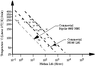
Temperature remains the most common stress variable, using the Arrhenius model for extrapolation. Figure A7.2 shows the temperature acceleration of infant mortality failures (see Section Four: Chapter 3 for a discussion on infant mortality).

Figure A7.2 An Arrhenius plot of bipolar and MOS infant mortality
data
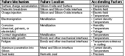
Many accelerating stresses besides elevated temperature activate various failure mechanisms. Such stresses include electric fields, current density, humidity, voltage, temperature extremes in cycling, and pressure. Table A7.1 lists several failure mechanisms, their device locations, and the factors that can be elevated to accelerate such failure mechanisms.

Table A7.1 Failure mechanisms, their locations and associated
accelerating factors
J. B. Bowles, "A survey of reliability-prediction procedures for microelectronic devices," IEEE Transactions on Reliability, Vol 41, No. 1, March 1992, pp. 4-11.
British Telecom, Handbook of Reliability Data for Components Used in Telecommunications Systems, Issue 4, January 1987.
Centre National D'Etudes des Telecommunications, Recueil De Donnees De Fiabilite Du CNET ( Collection of Reliability Data from CNET), 1983.
Department of Defense, MIL-HDBK-217, Reliability Prediction of Electronic Equipment, Department of Defense, Information Handling Services, Washington, D.C., December 1991.
Anthony J. Feduccia, IEEE Spectrum, Aug.,1992, pp. 46-49.
W. Feller, An introduction to probability theory and it applications, Vol. I, 1st ed., 1968 and Vol. II, 2d ed., 1970, Wiley, New York.
D. P. Holcomb, and J. C. North, "An infant mortality and long- term failure rate model for electronic equipment," AT & T Technical Journal 64, 1, 1985.
D. J. Klinger, Y. Nakada, M. Menendez, AT & T reliability manual, Van Nostrand Reinhold, New York, 1990.
W. Mendenhall, R. L. Schaeffer, D. D. Wackerly, Mathematical statistics with applications, 3d ed., Duxbury Press, Boston, 1986.
Nippon Telegraph and Telephone Corp., Standard reliability table for semiconductor devices, March, 1985.
P. D. T. O'Connor, Practical reliability engineering, 2nd ed., Wiley, New York, 1985.
M. L. Shooman, Probabilistic Reliability: An engineering approach, McGraw-Hill, New York, 1968.
Siemens Standard, SN29500, Reliability and quality specification failure rates of components, Siemens Standard, 1986.
G. F. Watson, "MIL Reliability: A new approach," IEEE Spectrum, Aug. 1992, pp. 46-49.
Now you may jump to: